Development and Validation of an Incompressible Navier-Stokes Solver – Part 1
Objectives
- Develop an incompressible Navier-Stokes solver using a fractional-step method and finite difference discretization to simulate viscous fluid flows.
- Validate the solver by simulating lid-driven cavity flow and comparing velocity profiles with benchmark data to assess accuracy.
- Apply the solver to simulate flow over a square obstacle at different Reynolds numbers to analyze wake formation, vortex shedding, and flow separation.
- Evaluate the solver’s performance and numerical stability by testing different boundary conditions, time-stepping methods, and solver configurations.
Governing Equations
The incompressible Navier-Stokes (iNS) equations governing viscous, incompressible fluid flow are given as:
\[\frac{\partial \mathbf{u}}{\partial t} + (\mathbf{u} \cdot \nabla) \mathbf{u} = -\frac{1}{\rho} \nabla p + \nu \nabla^2 \mathbf{u} + \mathbf{f}, \quad \nabla \cdot \mathbf{u} = 0\]where \(\mathbf{u}\) is the velocity field, \(p\) is pressure, \(\nu\) is kinematic viscosity, and \(\mathbf{f}\) represents external forces. To solve these equations, a fractional-step method is used with the Adams-Bashforth (AB2) scheme for advection and Crank-Nicolson (CN) scheme for diffusion.
The final discretized iNS equations, formulated by Perot, ensure second-order accuracy in time and are expressed as:
\[R u^F = S u^n + \Delta t \left( \frac{3a^n - a^{n-1}}{2} \right) + \frac{\Delta t \nu}{2} \left( bc_L^{n+1} + bc_L^n \right)\] \[D R^{-1} G P^{n+1} = \frac{D u^F}{\Delta t} + \frac{bc_D^{n+1}}{\Delta t}\] \[u^{n+1} = u^F - \Delta t R^{-1} G P^{n+1}\]where \(u^F\) is the fractional-step velocity, \(a^n\) is the advection term, and \(bc_L, bc_D\) are boundary condition terms. The operators are defined as:
\[R = I - \frac{\Delta t}{2} \nu L, \quad S = I + \frac{\Delta t}{2} \nu L, \quad R^{-1} \approx I + \frac{\Delta t}{2} \nu L\]where \(D, G, L\) represent the divergence, gradient, and Laplacian operators, respectively.
Grid and Domain Setup
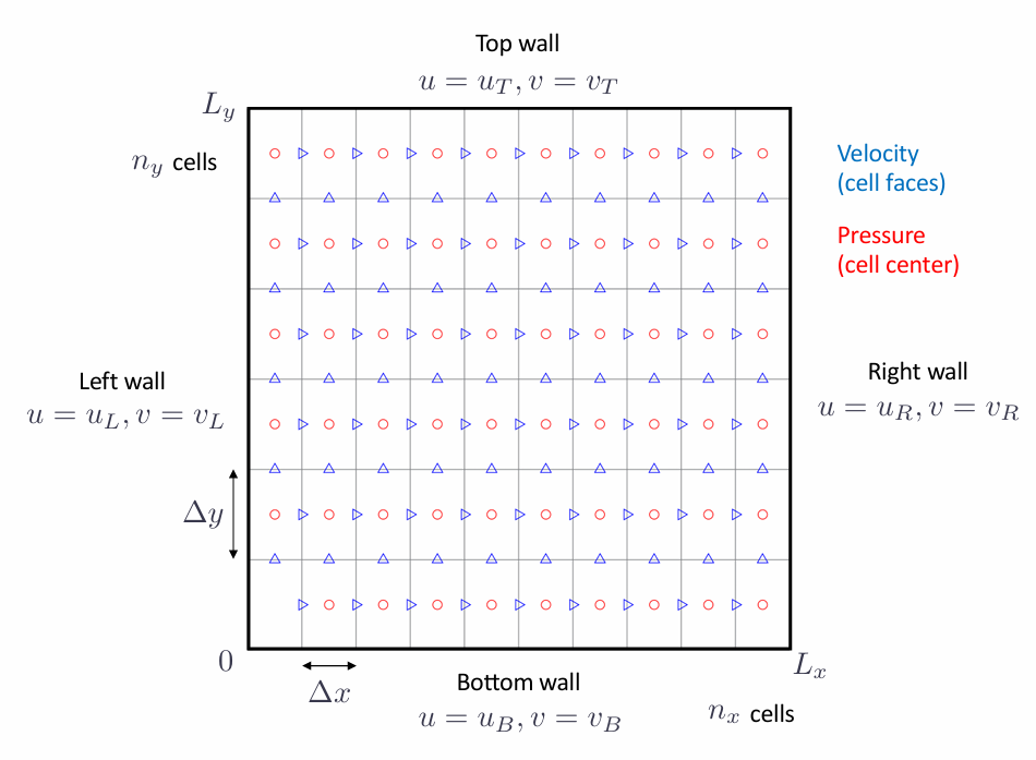
A staggered grid is used to discretize the domain, where velocity components \(u, v\) are stored at the cell faces, while pressure is stored at the cell centers. This approach helps prevent checkerboard instability, which occurs when using a regular grid for pressure and velocity storage.
The computational domain is a \(1 \times 1\) square discretized into a \(129 \times 129\) grid. The boundary conditions are as follows:
- Top boundary: \(u = 1\), \(v = 0\) (to simulate a moving lid).
- Bottom, left, and right boundaries: \(u = 0\), \(v = 0\) (stationary walls).
- Initial conditions: The velocity and pressure fields are initialized to zero.
A schematic representation of the staggered grid is shown below:
Solution Procedure
The solution begins with the creation of a pointer matrix system, which maps 2D velocity and pressure locations to a 1D index for efficient data handling. This matrix is used to construct key operators, including divergence, Laplacian, gradient, advection, and boundary condition vectors.
The simulation starts with zero initial conditions for velocity and pressure. The fractional-step algorithm is executed iteratively, with each time step consisting of:
- Velocity prediction step using a conjugate gradient solver.
- Pressure correction step to enforce incompressibility.
- Velocity update step via matrix operations.
A small time step is chosen to maintain numerical stability. The solver is validated against Ghia et al.’s benchmark results (Link) at \(Re = 100\), with a conjugate gradient solver tolerance of \(10^{-10}\) to ensure accuracy in solving the linear systems.
Results and Discussion
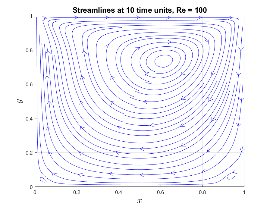
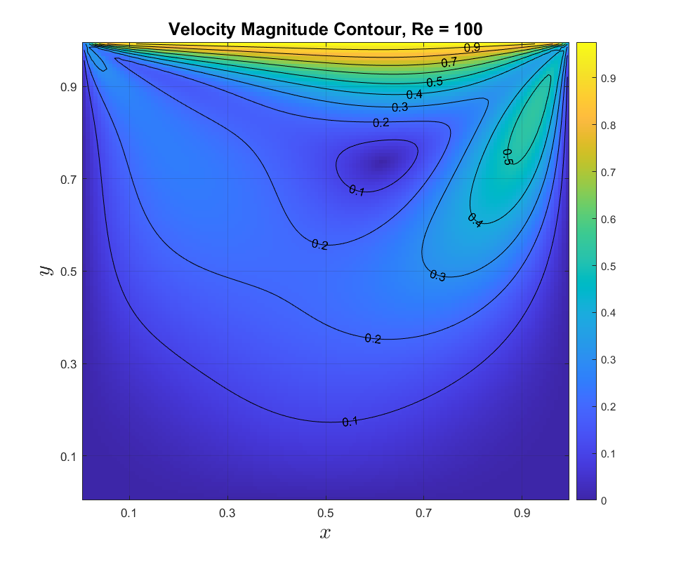
The streamline plot at \(Re = 100\) shows a dominant clockwise vortex in the cavity center, with secondary vortices near the bottom corners due to flow separation. These patterns align exactly with Ghia et al.’s benchmark results, confirming solver accuracy. Similar trends appear in the velocity magnitude contours.
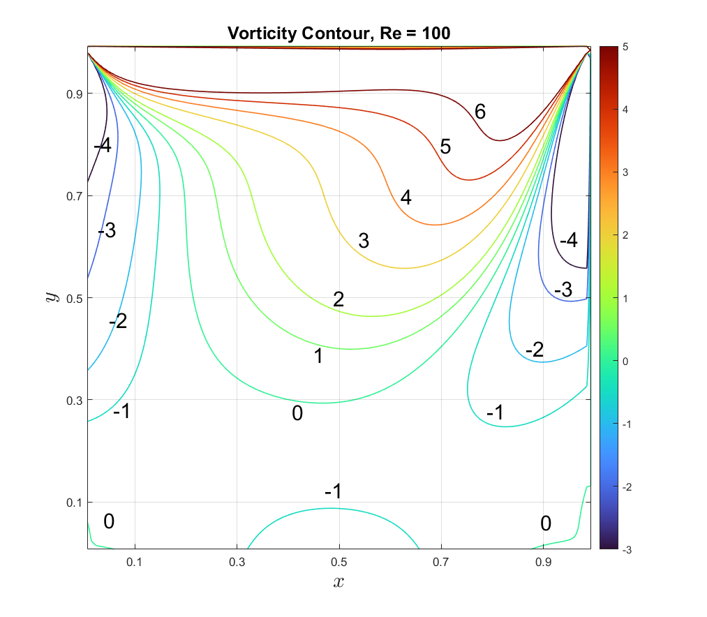
The vorticity contours reveal strong shear forces near the top boundary due to lid motion, with values ranging from \(-4\) to \(+6\). The contours and values match exactly with Ghia et al., demonstrating the solver’s ability to accurately capture vorticity transport.
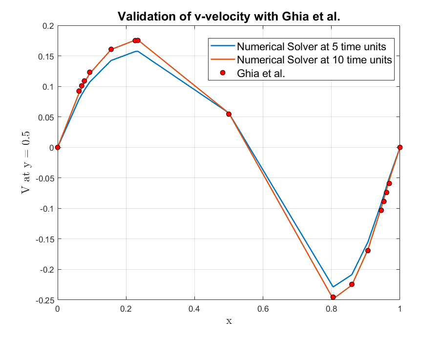
Validation against Ghia et al.’s velocity profiles shows minor deviations at 5 time units, particularly in steep gradient regions, but by 10 time units, the numerical solution fully converges to the benchmark data, confirming solver reliability.