Extending the Incompressible Solver for Flow Over a Square Geometry – Part 2

Introduction and Domain Setup

The incompressible Navier-Stokes solver is extended to simulate flow over a square cylinder. The computational domain is \(3 \times 1\), discretized with a \(301 \times 101\) grid. The square obstacle, located from \(x = 0.5\) to \(x = 0.7\), \(y = 0.4\) to \(y = 0.6\), is embedded within the domain.

Boundary Conditions:

• Inlet (Left Boundary): Dirichlet conditions, \(u = 1, v = 0\) (uniform inflow).
• Top and Bottom Boundary: Dirichlet conditions, \(u = 1, v = 0\) (uniform inflow).
• Square Surface: No-slip conditions, \(u = 0, v = 0\).
• Outlet (Right Boundary): Dirichlet condition, \(u = 1, v = 0\).

While Dirichlet conditions are used at the outlet, they are not ideal for unsteady flows. Neumann or Convective Boundary Conditions (CBC) are often preferred, but an attempt to implement Neumann conditions resulted in numerical instability and solver divergence.

A small time step is used to maintain numerical stability and accurately capture flow dynamics around the square geometry.

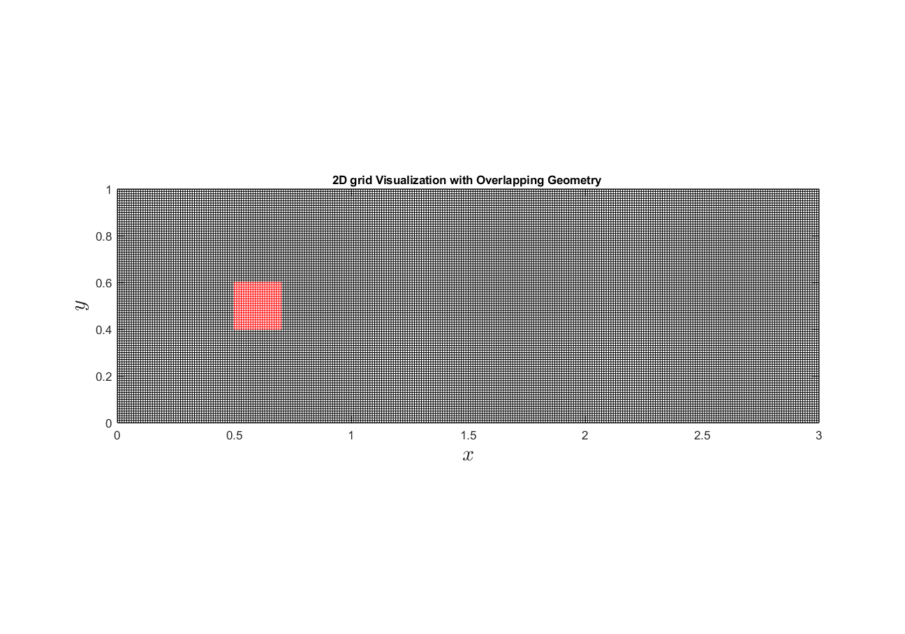
Solution Procedure

To incorporate the effect of the square obstacle within the computational domain, the solver first identifies the square’s boundary locations in both the x- and y-directions. Using this information, the numerical operators are modified to correctly account for the presence of the square.

Whenever an operator attempts to compute a value at a cell inside the square, the calculation is skipped, effectively treating the interior as a solid region. For boundary points near the square, the numerical treatment depends on whether the calculation involves locations adjacent to the square boundary, such as pressure nodes at cell centers, or directly on the square surface, such as velocity components at cell faces.

The pressure gradient is computed at velocity locations, which correspond to cell faces. At the square surface, the pressure gradient is set to zero, enforcing a homogeneous Neumann boundary condition. This ensures no flux normal to the surface, maintaining the no-penetration condition at the walls.

By carefully implementing these modifications, the solver accurately represents the effect of the square obstacle, ensuring that the boundary conditions and flow physics are properly captured in the simulation.

Characteristics of Cylinder Wake Across Reynolds Number Regimes

The wake behavior behind a square obstacle changes significantly with increasing Reynolds number (Re), defined as:

where \(U_{\infty}\) is the free-stream velocity, \(D\) is the cylinder width, and \(\nu\) is the kinematic viscosity.

For \(Re < 50\), the flow remains steady and laminar, forming symmetric recirculation bubbles. At \(50 < Re < 200\), laminar vortex shedding begins, forming a von Kármán vortex street, with decreasing vortex formation length and increasing Strouhal number \(( St )\).

For \(200 ≲ Re ≲ 260\), the wake transitions to 3D, further enhancing three-dimensionality as Re increases. At \(10^3 < Re < 2 \times 10^5\), the shear layer becomes turbulent, reducing vortex formation length while \(St\) decreases.

A critical transition occurs at \(2 \times 10^5 < Re < 4 \times 10^5\), where the shear layer approaches separation, causing a sudden drop in drag and a sharp rise in \(St\). At \(Re > 4 × 10^5\), the boundary layer fully transitions to turbulence, marking the post-critical regime.

These transitions highlight the impact of \(Re\) on wake structures, affecting fluid forces and vortex dynamics.

Results and Discussion

Part 1: Flow Evolution at Fixed Reynolds Number (Re = 1500) Over Time

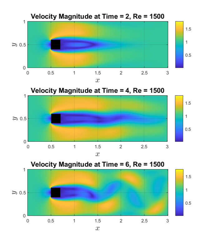
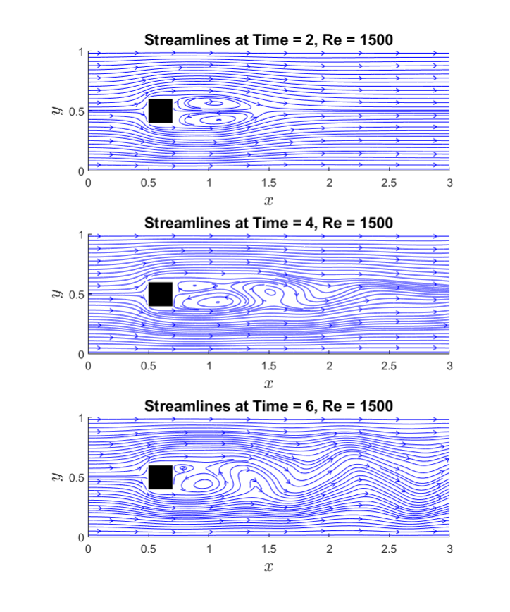
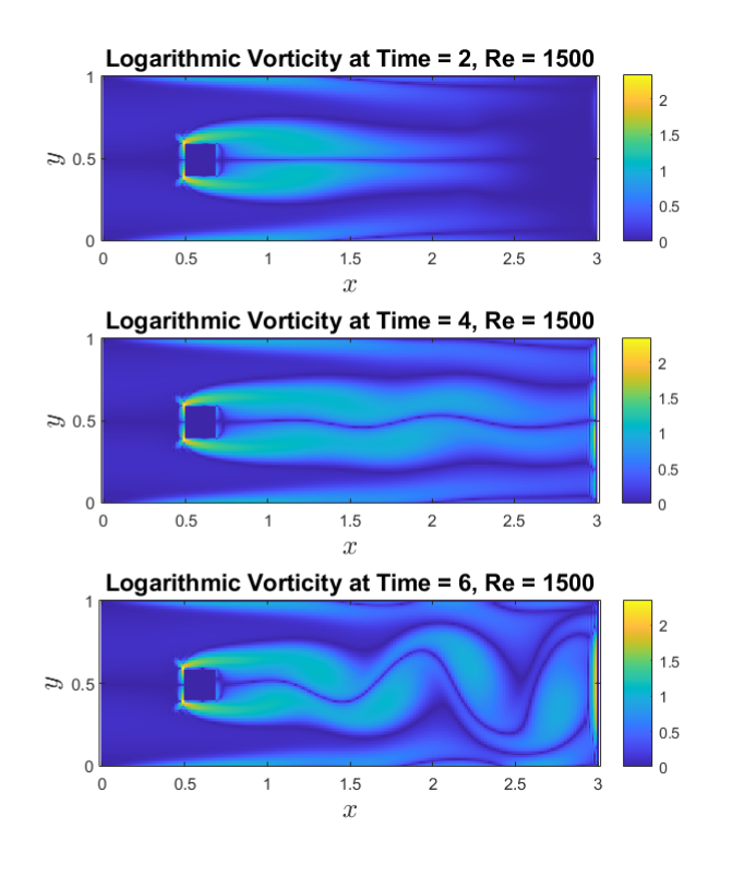
The time evolution of flow at \(Re = 1500\) is analyzed using velocity magnitude, streamlines, and vorticity contours at \(t = 2, t = 4,\) and \(t = 6\).

At \(t = 2\), strong acceleration near the leading edges of the square creates well-defined shear layers. The wake remains short and symmetric, with low-velocity regions concentrated in the center. By \(t = 4\), the wake elongates, and vortex shedding begins, forming alternating high- and low-velocity regions. At \(t = 6\), the wake reaches a quasi-periodic state, with a fully developed von Kármán vortex street, where alternating vortices interact and enhance mixing.

Streamlines further illustrate this wake development. At \(t = 2\), the wake is short and symmetric, with recirculation zones near the trailing edges. By \(t = 4\), the wake becomes elongated and asymmetric, indicating the onset of vortex shedding. At \(t = 6\), a periodic von Kármán vortex street is fully formed, with distinct alternating vortices.

Vorticity contours highlight strong shear near square corners, where flow separation occurs. A logarithmic scale is used to better visualize high vorticity values near the obstacle and weaker vorticity in the wake. At \(t = 2\), the wake is mostly symmetric, but by \(t = 4\), alternating vortices become more prominent, leading to a fully developed vortex street at \(t = 6\). Irregularities near the outlet arise due to imposed Dirichlet boundary conditions, but the overall wake structure is accurately captured.

Part 2: Flow Behavior at Different Reynolds Numbers at a Fixed Time (t = 4)

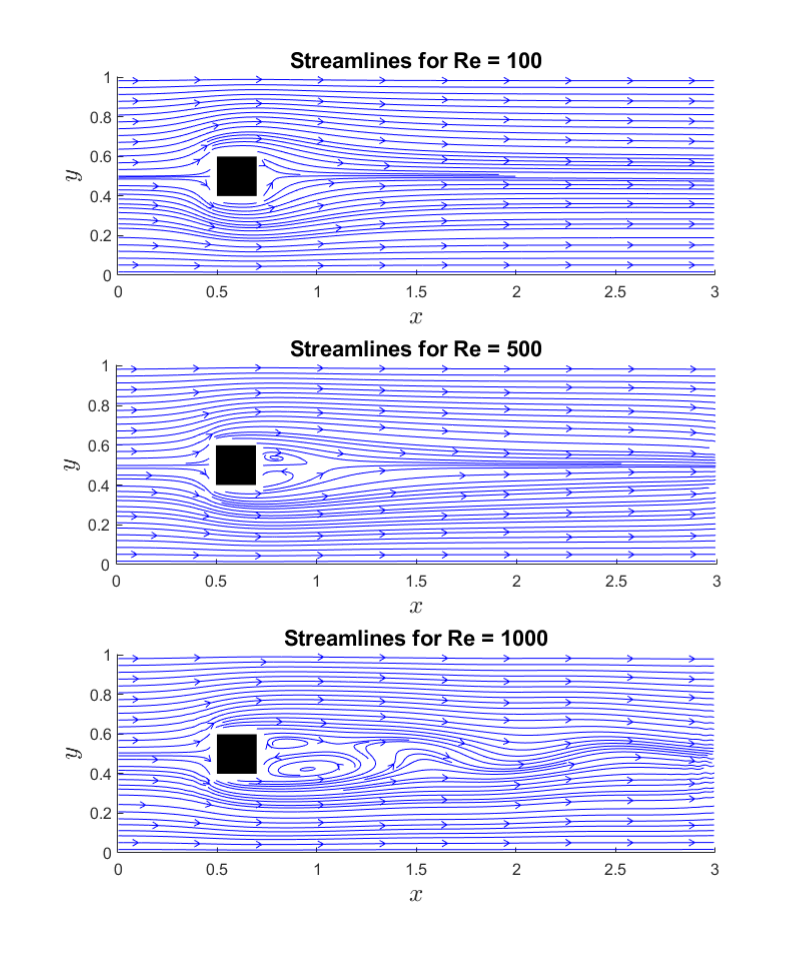
The wake dynamics around the square obstacle at \(t = 4\) are analyzed for different Reynolds numbers (\(Re = 100, 500, 1000, 1500, 2000, 5000, 10000\)). Streamline plots illustrate the transition from steady laminar flow at low \(Re\) to highly unsteady and turbulent wake patterns at higher \(Re\).

The figure shown below compares the flow for \(Re = 100, 500,\) and \(1000\). At \(Re = 100\), the flow remains laminar and steady, with symmetric recirculation bubbles forming directly downstream of the square. The wake region is short and well-defined, with minimal flow separation. At \(Re = 500\), the wake elongates, and the curvature of streamlines near the square’s trailing edges increases, indicating stronger flow separation. By \(Re = 1000\), the onset of vortex shedding appears, with alternating recirculation zones forming in the wake, marking the beginning of a von Kármán vortex street.

Finally, the figure shown below compares the wake structure at \(Re = 1500, 2000, 5000,\) and \(10000\). At \(Re = 1500\), vortex shedding is fully developed, with alternating vortices becoming more pronounced. At \(Re = 2000\), the wake length increases significantly, with stronger interactions between shear layers and the wake. At \(Re = 5000\), the flow transitions toward turbulence, displaying chaotic wake structures and irregular vortex shedding. By \(Re = 10000\), the wake is highly turbulent, characterized by intense mixing and the breakdown of coherent vortex structures. Flow separation near the square becomes substantial, and wake dynamics dominate the overall flow behavior.

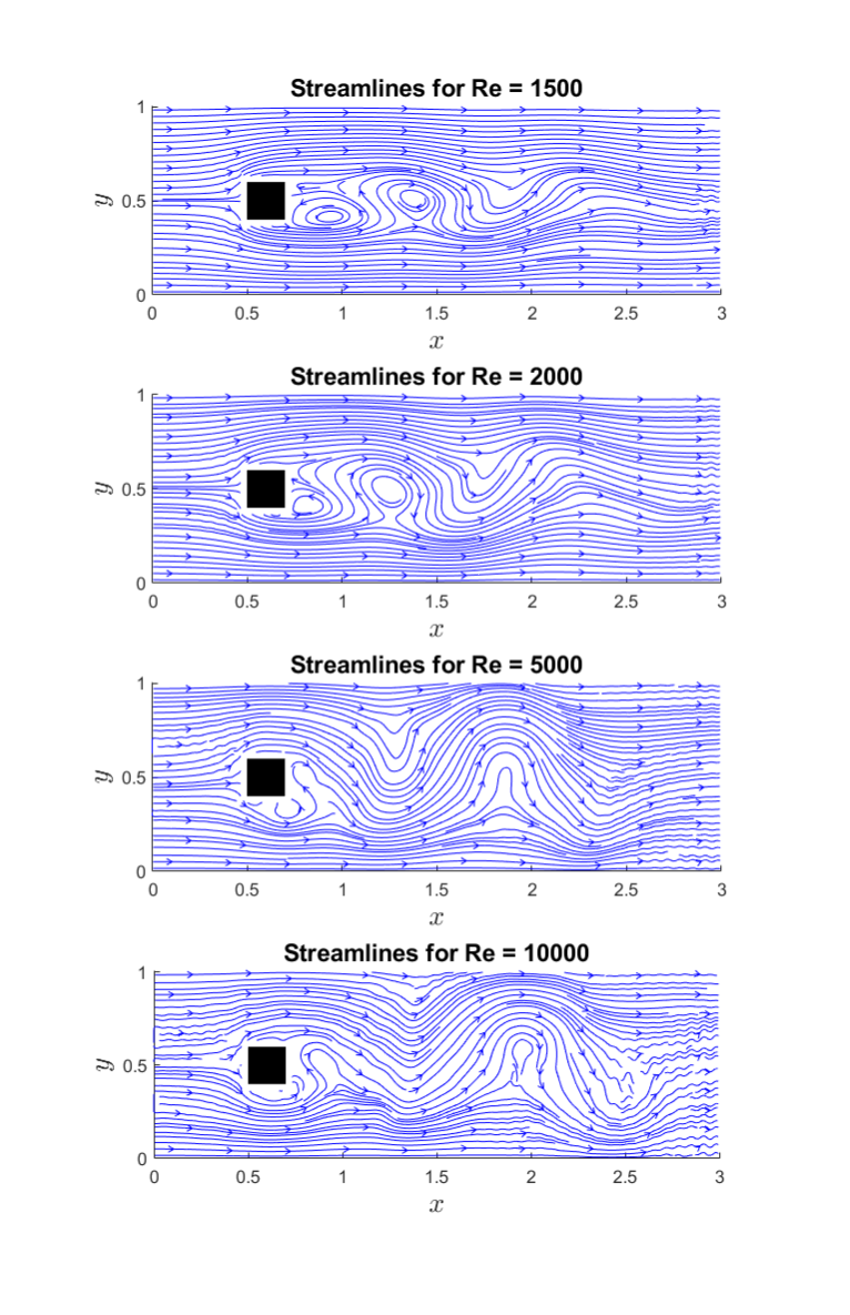
These figures collectively demonstrate the progressive transition from steady laminar flow to unsteady vortex shedding, ultimately leading to turbulent wake dynamics as \(Re\) increases.